resistics.spectra module#
Module containing functions and classes related to Spectra calculation and manipulation
Spectra are calculated from the windowed, decimated time data. The inbuilt Fourier transform implementation is inspired by the implementation of the scipy stft function.
- pydantic model resistics.spectra.SpectraLevelMetadata[source]#
Bases:
MetadataMetadata for spectra of a windowed decimation level
Show JSON schema
{
   "title": "SpectraLevelMetadata",
   "description": "Metadata for spectra of a windowed decimation level",
   "type": "object",
   "properties": {
      "fs": {
         "title": "Fs",
         "type": "number"
      },
      "n_wins": {
         "title": "N Wins",
         "type": "integer"
      },
      "win_size": {
         "title": "Win Size",
         "exclusiveMinimum": 0,
         "type": "integer"
      },
      "olap_size": {
         "title": "Olap Size",
         "exclusiveMinimum": 0,
         "type": "integer"
      },
      "index_offset": {
         "title": "Index Offset",
         "type": "integer"
      },
      "n_freqs": {
         "title": "N Freqs",
         "type": "integer"
      },
      "freqs": {
         "title": "Freqs",
         "type": "array",
         "items": {
            "type": "number"
         }
      }
   },
   "required": [
      "fs",
      "n_wins",
      "win_size",
      "olap_size",
      "index_offset",
      "n_freqs",
      "freqs"
   ]
}
- field win_size: PositiveInt [Required]#
The window size in samples
- Constraints:
exclusiveMinimum = 0
- field olap_size: PositiveInt [Required]#
The overlap size in samples
- Constraints:
exclusiveMinimum = 0
- pydantic model resistics.spectra.SpectraMetadata[source]#
Bases:
WriteableMetadataMetadata for spectra data
Show JSON schema
{
   "title": "SpectraMetadata",
   "description": "Metadata for spectra data",
   "type": "object",
   "properties": {
      "file_info": {
         "$ref": "#/definitions/ResisticsFile"
      },
      "fs": {
         "title": "Fs",
         "type": "array",
         "items": {
            "type": "number"
         }
      },
      "chans": {
         "title": "Chans",
         "type": "array",
         "items": {
            "type": "string"
         }
      },
      "n_chans": {
         "title": "N Chans",
         "type": "integer"
      },
      "n_levels": {
         "title": "N Levels",
         "type": "integer"
      },
      "first_time": {
         "title": "First Time",
         "pattern": "%Y-%m-%d %H:%M:%S.%f_%o_%q_%v",
         "examples": [
            "2021-01-01 00:00:00.000061_035156_250000_000000"
         ]
      },
      "last_time": {
         "title": "Last Time",
         "pattern": "%Y-%m-%d %H:%M:%S.%f_%o_%q_%v",
         "examples": [
            "2021-01-01 00:00:00.000061_035156_250000_000000"
         ]
      },
      "system": {
         "title": "System",
         "default": "",
         "type": "string"
      },
      "serial": {
         "title": "Serial",
         "default": "",
         "type": "string"
      },
      "wgs84_latitude": {
         "title": "Wgs84 Latitude",
         "default": -999.0,
         "type": "number"
      },
      "wgs84_longitude": {
         "title": "Wgs84 Longitude",
         "default": -999.0,
         "type": "number"
      },
      "easting": {
         "title": "Easting",
         "default": -999.0,
         "type": "number"
      },
      "northing": {
         "title": "Northing",
         "default": -999.0,
         "type": "number"
      },
      "elevation": {
         "title": "Elevation",
         "default": -999.0,
         "type": "number"
      },
      "chans_metadata": {
         "title": "Chans Metadata",
         "type": "object",
         "additionalProperties": {
            "$ref": "#/definitions/ChanMetadata"
         }
      },
      "levels_metadata": {
         "title": "Levels Metadata",
         "type": "array",
         "items": {
            "$ref": "#/definitions/SpectraLevelMetadata"
         }
      },
      "ref_time": {
         "title": "Ref Time",
         "pattern": "%Y-%m-%d %H:%M:%S.%f_%o_%q_%v",
         "examples": [
            "2021-01-01 00:00:00.000061_035156_250000_000000"
         ]
      },
      "history": {
         "title": "History",
         "default": {
            "records": []
         },
         "allOf": [
            {
               "$ref": "#/definitions/History"
            }
         ]
      }
   },
   "required": [
      "fs",
      "chans",
      "n_levels",
      "first_time",
      "last_time",
      "chans_metadata",
      "levels_metadata",
      "ref_time"
   ],
   "definitions": {
      "ResisticsFile": {
         "title": "ResisticsFile",
         "description": "Required information for writing out a resistics file",
         "type": "object",
         "properties": {
            "created_on_local": {
               "title": "Created On Local",
               "type": "string",
               "format": "date-time"
            },
            "created_on_utc": {
               "title": "Created On Utc",
               "type": "string",
               "format": "date-time"
            },
            "version": {
               "title": "Version",
               "type": "string"
            }
         }
      },
      "ChanMetadata": {
         "title": "ChanMetadata",
         "description": "Channel metadata",
         "type": "object",
         "properties": {
            "name": {
               "title": "Name",
               "type": "string"
            },
            "data_files": {
               "title": "Data Files",
               "type": "array",
               "items": {
                  "type": "string"
               }
            },
            "chan_type": {
               "title": "Chan Type",
               "type": "string"
            },
            "chan_source": {
               "title": "Chan Source",
               "type": "string"
            },
            "sensor": {
               "title": "Sensor",
               "default": "",
               "type": "string"
            },
            "serial": {
               "title": "Serial",
               "default": "",
               "type": "string"
            },
            "gain1": {
               "title": "Gain1",
               "default": 1,
               "type": "number"
            },
            "gain2": {
               "title": "Gain2",
               "default": 1,
               "type": "number"
            },
            "scaling": {
               "title": "Scaling",
               "default": 1,
               "type": "number"
            },
            "chopper": {
               "title": "Chopper",
               "default": false,
               "type": "boolean"
            },
            "dipole_dist": {
               "title": "Dipole Dist",
               "default": 1,
               "type": "number"
            },
            "sensor_calibration_file": {
               "title": "Sensor Calibration File",
               "default": "",
               "type": "string"
            },
            "instrument_calibration_file": {
               "title": "Instrument Calibration File",
               "default": "",
               "type": "string"
            }
         },
         "required": [
            "name"
         ]
      },
      "SpectraLevelMetadata": {
         "title": "SpectraLevelMetadata",
         "description": "Metadata for spectra of a windowed decimation level",
         "type": "object",
         "properties": {
            "fs": {
               "title": "Fs",
               "type": "number"
            },
            "n_wins": {
               "title": "N Wins",
               "type": "integer"
            },
            "win_size": {
               "title": "Win Size",
               "exclusiveMinimum": 0,
               "type": "integer"
            },
            "olap_size": {
               "title": "Olap Size",
               "exclusiveMinimum": 0,
               "type": "integer"
            },
            "index_offset": {
               "title": "Index Offset",
               "type": "integer"
            },
            "n_freqs": {
               "title": "N Freqs",
               "type": "integer"
            },
            "freqs": {
               "title": "Freqs",
               "type": "array",
               "items": {
                  "type": "number"
               }
            }
         },
         "required": [
            "fs",
            "n_wins",
            "win_size",
            "olap_size",
            "index_offset",
            "n_freqs",
            "freqs"
         ]
      },
      "Record": {
         "title": "Record",
         "description": "Class to hold a record\n\nA record holds information about a process that was run. It is intended to\ntrack processes applied to data, allowing a process history to be saved\nalong with any datasets.\n\nExamples\n--------\nA simple example of creating a process record\n\n>>> from resistics.common import Record\n>>> messages = [\"message 1\", \"message 2\"]\n>>> record = Record(\n...     creator={\"name\": \"example\", \"parameter1\": 15},\n...     messages=messages,\n...     record_type=\"example\"\n... )\n>>> record.summary()\n{\n    'time_local': '...',\n    'time_utc': '...',\n    'creator': {'name': 'example', 'parameter1': 15},\n    'messages': ['message 1', 'message 2'],\n    'record_type': 'example'\n}",
         "type": "object",
         "properties": {
            "time_local": {
               "title": "Time Local",
               "type": "string",
               "format": "date-time"
            },
            "time_utc": {
               "title": "Time Utc",
               "type": "string",
               "format": "date-time"
            },
            "creator": {
               "title": "Creator",
               "type": "object"
            },
            "messages": {
               "title": "Messages",
               "type": "array",
               "items": {
                  "type": "string"
               }
            },
            "record_type": {
               "title": "Record Type",
               "type": "string"
            }
         },
         "required": [
            "creator",
            "messages",
            "record_type"
         ]
      },
      "History": {
         "title": "History",
         "description": "Class for storing processing history\n\nParameters\n----------\nrecords : List[Record], optional\n    List of records, by default []\n\nExamples\n--------\n>>> from resistics.testing import record_example1, record_example2\n>>> from resistics.common import History\n>>> record1 = record_example1()\n>>> record2 = record_example2()\n>>> history = History(records=[record1, record2])\n>>> history.summary()\n{\n    'records': [\n        {\n            'time_local': '...',\n            'time_utc': '...',\n            'creator': {\n                'name': 'example1',\n                'a': 5,\n                'b': -7.0\n            },\n            'messages': ['Message 1', 'Message 2'],\n            'record_type': 'process'\n        },\n        {\n            'time_local': '...',\n            'time_utc': '...',\n            'creator': {\n                'name': 'example2',\n                'a': 'parzen',\n                'b': -21\n            },\n            'messages': ['Message 5', 'Message 6'],\n            'record_type': 'process'\n        }\n    ]\n}",
         "type": "object",
         "properties": {
            "records": {
               "title": "Records",
               "default": [],
               "type": "array",
               "items": {
                  "$ref": "#/definitions/Record"
               }
            }
         }
      }
   }
}
- field first_time: HighResDateTime [Required]#
- Constraints:
pattern = %Y-%m-%d %H:%M:%S.%f_%o_%q_%v
examples = [‘2021-01-01 00:00:00.000061_035156_250000_000000’]
- field last_time: HighResDateTime [Required]#
- Constraints:
pattern = %Y-%m-%d %H:%M:%S.%f_%o_%q_%v
examples = [‘2021-01-01 00:00:00.000061_035156_250000_000000’]
- field chans_metadata: Dict[str, ChanMetadata] [Required]#
- field levels_metadata: List[SpectraLevelMetadata] [Required]#
- field ref_time: HighResDateTime [Required]#
- Constraints:
pattern = %Y-%m-%d %H:%M:%S.%f_%o_%q_%v
examples = [‘2021-01-01 00:00:00.000061_035156_250000_000000’]
- class resistics.spectra.SpectraData(metadata: SpectraMetadata, data: Dict[int, ndarray])[source]#
Bases:
ResisticsDataClass for holding spectra data
The spectra data is stored in the class as a dictionary mapping decimation level to numpy array. The shape of the array for each decimation level is:
n_wins x n_chans x n_freqs
- get_chan(level: int, chan: str) ndarray[source]#
Get the channel spectra data for a decimation level
- get_chans(level: int, chans: List[str]) ndarray[source]#
Get the channels spectra data for a decimation level
- get_freq(level: int, idx: int) ndarray[source]#
Get the spectra data at a frequency index for a decimation level
- get_mag_phs(level: int, unwrap: bool = False) Tuple[ndarray, ndarray][source]#
Get magnitude and phase for a decimation level
- get_timestamps(level: int) DatetimeIndex[source]#
Get the start time of each window
Note that this does not use high resolution timestamps
- Parameters:
level (int) – The decimation level
- Returns:
The starts of each window
- Return type:
pd.DatetimeIndex
- Raises:
ValueError – If the level is out of range
- plot(max_pts: int | None = 10000) Figure[source]#
Stack spectra data for all decimation levels
- Parameters:
max_pts (Optional[int], optional) – The maximum number of points in any individual plot before applying lttbc downsampling, by default 10_000. If set to None, no downsampling will be applied.
- Returns:
The plotly figure
- Return type:
go.Figure
- plot_level_stack(level: int, max_pts: int = 10000, grouping: str | None = None, offset: str = '0h') Figure[source]#
Stack the spectra for a decimation level with optional time grouping
- Parameters:
level (int) – The decimation level
max_pts (int, optional) – The maximum number of points in any individual plot before applying lttbc downsampling, by default 10_000
grouping (Optional[str], optional) – A grouping interval as a pandas freq string, by default None
offset (str, optional) – A time offset to add to the grouping, by default “0h”. For instance, to plot night time and day time spectra, set grouping to “12h” and offset to “6h”
- Returns:
The plotly figure
- Return type:
go.Figure
- pydantic model resistics.spectra.FourierTransform[source]#
Bases:
ResisticsProcessPerform a Fourier transform of the windowed data
The processor is inspired by the scipy.signal.stft function which performs a similar process and involves a Fourier transform along the last axis of the windowed data.
- Parameters:
win_fnc (Union[str, Tuple[str, float]]) – The window to use before performing the FFT, by default (“kaiser”, 14)
detrend (Union[str, None]) – Type of detrending to apply before performing FFT, by default linear detrend. Setting to None will not apply any detrending to the data prior to the FFT
workers (int) – The number of CPUs to use, by default max - 2
Examples
This example will get periodic decimated data, perfrom windowing and run the Fourier transform on the windowed data.
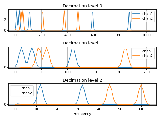
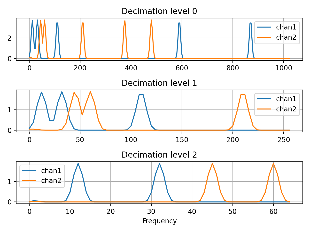
>>> import matplotlib.pyplot as plt
>>> import numpy as np
>>> from resistics.testing import decimated_data_periodic
>>> from resistics.window import WindowSetup, Windower
>>> from resistics.spectra import FourierTransform
>>> frequencies = {"chan1": [870, 590, 110, 32, 12], "chan2": [480, 375, 210, 60, 45]}
>>> dec_data = decimated_data_periodic(frequencies, fs=128)
>>> dec_data.metadata.chans
['chan1', 'chan2']
>>> print(dec_data.to_string())
<class 'resistics.decimate.DecimatedData'>
           fs        dt  n_samples           first_time                        last_time
level
0      2048.0  0.000488      16384  2021-01-01 00:00:00  2021-01-01 00:00:07.99951171875
1       512.0  0.001953       4096  2021-01-01 00:00:00    2021-01-01 00:00:07.998046875
2       128.0  0.007812       1024  2021-01-01 00:00:00      2021-01-01 00:00:07.9921875
Perform the windowing
>>> win_params = WindowSetup().run(dec_data.metadata.n_levels, dec_data.metadata.fs)
>>> win_data = Windower().run(dec_data.metadata.first_time, win_params, dec_data)
And then the Fourier transform. By default, the data will be (linearly) detrended and mutliplied by a Kaiser window prior to the Fourier transform
>>> spec_data = FourierTransform().run(win_data)
For plotting of magnitude, let’s stack the spectra
>>> freqs_0 = spec_data.metadata.levels_metadata[0].freqs
>>> data_0 = np.absolute(spec_data.data[0]).mean(axis=0)
>>> freqs_1 = spec_data.metadata.levels_metadata[1].freqs
>>> data_1 = np.absolute(spec_data.data[1]).mean(axis=0)
>>> freqs_2 = spec_data.metadata.levels_metadata[2].freqs
>>> data_2 = np.absolute(spec_data.data[2]).mean(axis=0)
Now plot
>>> plt.subplot(3,1,1)
>>> plt.plot(freqs_0, data_0[0], label="chan1")
>>> plt.plot(freqs_0, data_0[1], label="chan2")
>>> plt.grid()
>>> plt.title("Decimation level 0")
>>> plt.legend()
>>> plt.subplot(3,1,2)
>>> plt.plot(freqs_1, data_1[0], label="chan1")
>>> plt.plot(freqs_1, data_1[1], label="chan2")
>>> plt.grid()
>>> plt.title("Decimation level 1")
>>> plt.legend()
>>> plt.subplot(3,1,3)
>>> plt.plot(freqs_2, data_2[0], label="chan1")
>>> plt.plot(freqs_2, data_2[1], label="chan2")
>>> plt.grid()
>>> plt.title("Decimation level 2")
>>> plt.legend()
>>> plt.xlabel("Frequency")
>>> plt.tight_layout()
>>> plt.show()
(
Source code,png,hires.png,pdf)
Show JSON schema
{
   "title": "FourierTransform",
   "description": "Perform a Fourier transform of the windowed data\n\nThe processor is inspired by the scipy.signal.stft function which performs\na similar process and involves a Fourier transform along the last axis of\nthe windowed data.\n\nParameters\n----------\nwin_fnc : Union[str, Tuple[str, float]]\n    The window to use before performing the FFT, by default (\"kaiser\", 14)\ndetrend : Union[str, None]\n    Type of detrending to apply before performing FFT, by default linear\n    detrend. Setting to None will not apply any detrending to the data prior\n    to the FFT\nworkers : int\n    The number of CPUs to use, by default max - 2\n\nExamples\n--------\nThis example will get periodic decimated data, perfrom windowing and run the\nFourier transform on the windowed data.\n\n.. plot::\n    :width: 90%\n\n    >>> import matplotlib.pyplot as plt\n    >>> import numpy as np\n    >>> from resistics.testing import decimated_data_periodic\n    >>> from resistics.window import WindowSetup, Windower\n    >>> from resistics.spectra import FourierTransform\n    >>> frequencies = {\"chan1\": [870, 590, 110, 32, 12], \"chan2\": [480, 375, 210, 60, 45]}\n    >>> dec_data = decimated_data_periodic(frequencies, fs=128)\n    >>> dec_data.metadata.chans\n    ['chan1', 'chan2']\n    >>> print(dec_data.to_string())\n    <class 'resistics.decimate.DecimatedData'>\n               fs        dt  n_samples           first_time                        last_time\n    level\n    0      2048.0  0.000488      16384  2021-01-01 00:00:00  2021-01-01 00:00:07.99951171875\n    1       512.0  0.001953       4096  2021-01-01 00:00:00    2021-01-01 00:00:07.998046875\n    2       128.0  0.007812       1024  2021-01-01 00:00:00      2021-01-01 00:00:07.9921875\n\n    Perform the windowing\n\n    >>> win_params = WindowSetup().run(dec_data.metadata.n_levels, dec_data.metadata.fs)\n    >>> win_data = Windower().run(dec_data.metadata.first_time, win_params, dec_data)\n\n    And then the Fourier transform. By default, the data will be (linearly)\n    detrended and mutliplied by a Kaiser window prior to the Fourier\n    transform\n\n    >>> spec_data = FourierTransform().run(win_data)\n\n    For plotting of magnitude, let's stack the spectra\n\n    >>> freqs_0 = spec_data.metadata.levels_metadata[0].freqs\n    >>> data_0 = np.absolute(spec_data.data[0]).mean(axis=0)\n    >>> freqs_1 = spec_data.metadata.levels_metadata[1].freqs\n    >>> data_1 = np.absolute(spec_data.data[1]).mean(axis=0)\n    >>> freqs_2 = spec_data.metadata.levels_metadata[2].freqs\n    >>> data_2 = np.absolute(spec_data.data[2]).mean(axis=0)\n\n    Now plot\n\n    >>> plt.subplot(3,1,1) # doctest: +SKIP\n    >>> plt.plot(freqs_0, data_0[0], label=\"chan1\") # doctest: +SKIP\n    >>> plt.plot(freqs_0, data_0[1], label=\"chan2\") # doctest: +SKIP\n    >>> plt.grid()\n    >>> plt.title(\"Decimation level 0\") # doctest: +SKIP\n    >>> plt.legend() # doctest: +SKIP\n    >>> plt.subplot(3,1,2) # doctest: +SKIP\n    >>> plt.plot(freqs_1, data_1[0], label=\"chan1\") # doctest: +SKIP\n    >>> plt.plot(freqs_1, data_1[1], label=\"chan2\") # doctest: +SKIP\n    >>> plt.grid()\n    >>> plt.title(\"Decimation level 1\") # doctest: +SKIP\n    >>> plt.legend() # doctest: +SKIP\n    >>> plt.subplot(3,1,3) # doctest: +SKIP\n    >>> plt.plot(freqs_2, data_2[0], label=\"chan1\") # doctest: +SKIP\n    >>> plt.plot(freqs_2, data_2[1], label=\"chan2\") # doctest: +SKIP\n    >>> plt.grid()\n    >>> plt.title(\"Decimation level 2\") # doctest: +SKIP\n    >>> plt.legend() # doctest: +SKIP\n    >>> plt.xlabel(\"Frequency\") # doctest: +SKIP\n    >>> plt.tight_layout() # doctest: +SKIP\n    >>> plt.show() # doctest: +SKIP",
   "type": "object",
   "properties": {
      "name": {
         "title": "Name",
         "type": "string"
      },
      "win_fnc": {
         "title": "Win Fnc",
         "default": [
            "kaiser",
            14
         ],
         "anyOf": [
            {
               "type": "string"
            },
            {
               "type": "array",
               "minItems": 2,
               "maxItems": 2,
               "items": [
                  {
                     "type": "string"
                  },
                  {
                     "type": "number"
                  }
               ]
            }
         ]
      },
      "detrend": {
         "title": "Detrend",
         "default": "linear",
         "type": "string"
      },
      "workers": {
         "title": "Workers",
         "default": -2,
         "type": "integer"
      }
   }
}
- run(win_data: WindowedData) SpectraData[source]#
Perform the FFT
Data is padded to the next fast length before performing the FFT to speed up processing. Therefore, the output length may not be as expected.
- Parameters:
win_data (WindowedData) – The input windowed data
- Returns:
The Fourier transformed output
- Return type:
- pydantic model resistics.spectra.EvaluationFreqs[source]#
Bases:
ResisticsProcessCalculate the spectra values at the evaluation frequencies
This is done using linear interpolation in the complex domain
Example
The example will show interpolation to evaluation frequencies on a very simple example. Begin by generating some example spectra data.
>>> from resistics.decimate import DecimationSetup
>>> from resistics.spectra import EvaluationFreqs
>>> from resistics.testing import spectra_data_basic
>>> spec_data = spectra_data_basic()
>>> spec_data.metadata.n_levels
1
>>> spec_data.metadata.chans
['chan1']
>>> spec_data.metadata.levels_metadata[0].summary()
{
    'fs': 180.0,
    'n_wins': 2,
    'win_size': 20,
    'olap_size': 5,
    'index_offset': 0,
    'n_freqs': 10,
    'freqs': [0.0, 10.0, 20.0, 30.0, 40.0, 50.0, 60.0, 70.0, 80.0, 90.0]
}
The spectra data has only a single channel and a single level which has 2 windows. Now define our evaluation frequencies.
>>> eval_freqs = [1, 12, 23, 34, 45, 56, 67, 78, 89]
>>> dec_setup = DecimationSetup(n_levels=1, per_level=9, eval_freqs=eval_freqs)
>>> dec_params = dec_setup.run(spec_data.metadata.fs[0])
>>> dec_params.summary()
{
    'fs': 180.0,
    'n_levels': 1,
    'per_level': 9,
    'min_samples': 256,
    'eval_freqs': [1.0, 12.0, 23.0, 34.0, 45.0, 56.0, 67.0, 78.0, 89.0],
    'dec_factors': [1],
    'dec_increments': [1],
    'dec_fs': [180.0]
}
Now calculate the spectra at the evaluation frequencies
>>> eval_data = EvaluationFreqs().run(dec_params, spec_data)
>>> eval_data.metadata.levels_metadata[0].summary()
{
    'fs': 180.0,
    'n_wins': 2,
    'win_size': 20,
    'olap_size': 5,
    'index_offset': 0,
    'n_freqs': 9,
    'freqs': [1.0, 12.0, 23.0, 34.0, 45.0, 56.0, 67.0, 78.0, 89.0]
}
To double check everything is as expected, let’s compare the data. Comparing window 1 gives
>>> print(spec_data.data[0][0, 0])
[0.+0.j 1.+1.j 2.+2.j 3.+3.j 4.+4.j 5.+5.j 6.+6.j 7.+7.j 8.+8.j 9.+9.j]
>>> print(eval_data.data[0][0, 0])
[0.1+0.1j 1.2+1.2j 2.3+2.3j 3.4+3.4j 4.5+4.5j 5.6+5.6j 6.7+6.7j 7.8+7.8j
 8.9+8.9j]
And window 2
>>> print(spec_data.data[0][1, 0])
[-1. +1.j  0. +2.j  1. +3.j  2. +4.j  3. +5.j  4. +6.j  5. +7.j  6. +8.j
  7. +9.j  8.+10.j]
>>> print(eval_data.data[0][1, 0])
[-0.9+1.1j  0.2+2.2j  1.3+3.3j  2.4+4.4j  3.5+5.5j  4.6+6.6j  5.7+7.7j
  6.8+8.8j  7.9+9.9j]
Show JSON schema
{
   "title": "EvaluationFreqs",
   "description": "Calculate the spectra values at the evaluation frequencies\n\nThis is done using linear interpolation in the complex domain\n\nExample\n-------\nThe example will show interpolation to evaluation frequencies on a very\nsimple example. Begin by generating some example spectra data.\n\n>>> from resistics.decimate import DecimationSetup\n>>> from resistics.spectra import EvaluationFreqs\n>>> from resistics.testing import spectra_data_basic\n>>> spec_data = spectra_data_basic()\n>>> spec_data.metadata.n_levels\n1\n>>> spec_data.metadata.chans\n['chan1']\n>>> spec_data.metadata.levels_metadata[0].summary()\n{\n    'fs': 180.0,\n    'n_wins': 2,\n    'win_size': 20,\n    'olap_size': 5,\n    'index_offset': 0,\n    'n_freqs': 10,\n    'freqs': [0.0, 10.0, 20.0, 30.0, 40.0, 50.0, 60.0, 70.0, 80.0, 90.0]\n}\n\nThe spectra data has only a single channel and a single level which has 2\nwindows. Now define our evaluation frequencies.\n\n>>> eval_freqs = [1, 12, 23, 34, 45, 56, 67, 78, 89]\n>>> dec_setup = DecimationSetup(n_levels=1, per_level=9, eval_freqs=eval_freqs)\n>>> dec_params = dec_setup.run(spec_data.metadata.fs[0])\n>>> dec_params.summary()\n{\n    'fs': 180.0,\n    'n_levels': 1,\n    'per_level': 9,\n    'min_samples': 256,\n    'eval_freqs': [1.0, 12.0, 23.0, 34.0, 45.0, 56.0, 67.0, 78.0, 89.0],\n    'dec_factors': [1],\n    'dec_increments': [1],\n    'dec_fs': [180.0]\n}\n\nNow calculate the spectra at the evaluation frequencies\n\n>>> eval_data = EvaluationFreqs().run(dec_params, spec_data)\n>>> eval_data.metadata.levels_metadata[0].summary()\n{\n    'fs': 180.0,\n    'n_wins': 2,\n    'win_size': 20,\n    'olap_size': 5,\n    'index_offset': 0,\n    'n_freqs': 9,\n    'freqs': [1.0, 12.0, 23.0, 34.0, 45.0, 56.0, 67.0, 78.0, 89.0]\n}\n\nTo double check everything is as expected, let's compare the data. Comparing\nwindow 1 gives\n\n>>> print(spec_data.data[0][0, 0])\n[0.+0.j 1.+1.j 2.+2.j 3.+3.j 4.+4.j 5.+5.j 6.+6.j 7.+7.j 8.+8.j 9.+9.j]\n>>> print(eval_data.data[0][0, 0])\n[0.1+0.1j 1.2+1.2j 2.3+2.3j 3.4+3.4j 4.5+4.5j 5.6+5.6j 6.7+6.7j 7.8+7.8j\n 8.9+8.9j]\n\nAnd window 2\n\n>>> print(spec_data.data[0][1, 0])\n[-1. +1.j  0. +2.j  1. +3.j  2. +4.j  3. +5.j  4. +6.j  5. +7.j  6. +8.j\n  7. +9.j  8.+10.j]\n>>> print(eval_data.data[0][1, 0])\n[-0.9+1.1j  0.2+2.2j  1.3+3.3j  2.4+4.4j  3.5+5.5j  4.6+6.6j  5.7+7.7j\n  6.8+8.8j  7.9+9.9j]",
   "type": "object",
   "properties": {
      "name": {
         "title": "Name",
         "type": "string"
      }
   }
}
- run(dec_params: DecimationParameters, spec_data: SpectraData) SpectraData[source]#
Interpolate spectra data to the evaluation frequencies
This is a simple linear interpolation.
- Parameters:
dec_params (DecimationParameters) – The decimation parameters which have the evaluation frequencies for each decimation level
spec_data (SpectraData) – The spectra data
- Returns:
The spectra data at the evaluation frequencies
- Return type:
- pydantic model resistics.spectra.SpectraDataWriter[source]#
Bases:
ResisticsWriterWriter of resistics spectra data
Show JSON schema
{
   "title": "SpectraDataWriter",
   "description": "Writer of resistics spectra data",
   "type": "object",
   "properties": {
      "name": {
         "title": "Name",
         "type": "string"
      },
      "overwrite": {
         "title": "Overwrite",
         "default": true,
         "type": "boolean"
      }
   }
}
- run(dir_path: Path, spec_data: SpectraData) None[source]#
Write out SpectraData
- Parameters:
dir_path (Path) – The directory path to write to
spec_data (SpectraData) – Spectra data to write out
- Raises:
WriteError – If unable to write to the directory
- pydantic model resistics.spectra.SpectraDataReader[source]#
Bases:
ResisticsProcessReader of resistics spectra data
Show JSON schema
{
   "title": "SpectraDataReader",
   "description": "Reader of resistics spectra data",
   "type": "object",
   "properties": {
      "name": {
         "title": "Name",
         "type": "string"
      }
   }
}
- run(dir_path: Path, metadata_only: bool = False) SpectraMetadata | SpectraData[source]#
Read SpectraData
- Parameters:
dir_path (Path) – The directory path to read from
metadata_only (bool, optional) – Flag for getting metadata only, by default False
- Returns:
The SpectraData or SpectraMetadata if metadata_only is True
- Return type:
Union[SpectraMetadata, SpectraData]
- Raises:
ReadError – If the directory does not exist
- pydantic model resistics.spectra.SpectraProcess[source]#
Bases:
ResisticsProcessParent class for spectra processes
Show JSON schema
{
   "title": "SpectraProcess",
   "description": "Parent class for spectra processes",
   "type": "object",
   "properties": {
      "name": {
         "title": "Name",
         "type": "string"
      }
   }
}
- run(spec_data: SpectraData) SpectraData[source]#
Run a spectra processor
- pydantic model resistics.spectra.SpectraSmootherUniform[source]#
Bases:
SpectraProcessSmooth a spectra with a uniform filter
For more information, please refer to: https://docs.scipy.org/doc/scipy/reference/generated/scipy.ndimage.uniform_filter1d.html
Examples
Smooth a simple spectra data instance
>>> from resistics.spectra import SpectraSmootherUniform
>>> from resistics.testing import spectra_data_basic
>>> spec_data = spectra_data_basic()
>>> smooth_data = SpectraSmootherUniform(length_proportion=0.5).run(spec_data)
Look at the results for the two windows
>>> spec_data.data[0][0,0]
array([0.+0.j, 1.+1.j, 2.+2.j, 3.+3.j, 4.+4.j, 5.+5.j, 6.+6.j, 7.+7.j,
       8.+8.j, 9.+9.j])
>>> smooth_data.data[0][0,0]
array([0.8+0.8j, 1.2+1.2j, 2. +2.j , 3. +3.j , 4. +4.j , 5. +5.j ,
       6. +6.j , 7. +7.j , 7.8+7.8j, 8.2+8.2j])
Show JSON schema
{
   "title": "SpectraSmootherUniform",
   "description": "Smooth a spectra with a uniform filter\n\nFor more information, please refer to:\nhttps://docs.scipy.org/doc/scipy/reference/generated/scipy.ndimage.uniform_filter1d.html\n\nExamples\n--------\nSmooth a simple spectra data instance\n\n>>> from resistics.spectra import SpectraSmootherUniform\n>>> from resistics.testing import spectra_data_basic\n>>> spec_data = spectra_data_basic()\n>>> smooth_data = SpectraSmootherUniform(length_proportion=0.5).run(spec_data)\n\nLook at the results for the two windows\n\n>>> spec_data.data[0][0,0]\narray([0.+0.j, 1.+1.j, 2.+2.j, 3.+3.j, 4.+4.j, 5.+5.j, 6.+6.j, 7.+7.j,\n       8.+8.j, 9.+9.j])\n>>> smooth_data.data[0][0,0]\narray([0.8+0.8j, 1.2+1.2j, 2. +2.j , 3. +3.j , 4. +4.j , 5. +5.j ,\n       6. +6.j , 7. +7.j , 7.8+7.8j, 8.2+8.2j])",
   "type": "object",
   "properties": {
      "name": {
         "title": "Name",
         "type": "string"
      },
      "length_proportion": {
         "title": "Length Proportion",
         "default": 0.1,
         "type": "number"
      }
   }
}
- run(spec_data: SpectraData) SpectraData[source]#
Smooth spectra data with a uniform smoother
- Parameters:
spec_data (SpectraData) – The input spectra data
- Returns:
The output spectra data
- Return type:
- pydantic model resistics.spectra.SpectraSmootherGaussian[source]#
Bases:
SpectraProcessSmooth a spectra with a gaussian filter
For more information, please refer to: https://docs.scipy.org/doc/scipy/reference/generated/scipy.ndimage.gaussian_filter1d.html
Examples
Smooth a simple spectra data instance
>>> from resistics.spectra import SpectraSmootherGaussian
>>> from resistics.testing import spectra_data_basic
>>> spec_data = spectra_data_basic()
>>> smooth_data = SpectraSmootherGaussian().run(spec_data)
Look at the results for the two windows
>>> spec_data.data[0][0,0]
array([0.+0.j, 1.+1.j, 2.+2.j, 3.+3.j, 4.+4.j, 5.+5.j, 6.+6.j, 7.+7.j,
       8.+8.j, 9.+9.j])
>>> smooth_data.data[0][0,0]
array([1.93603671+1.93603671j, 2.1921536 +2.1921536j ,
       2.67507336+2.67507336j, 3.33255376+3.33255376j,
       4.09862656+4.09862656j, 4.90137344+4.90137344j,
       5.66744624+5.66744624j, 6.32492664+6.32492664j,
       6.8078464 +6.8078464j , 7.06396329+7.06396329j])
Show JSON schema
{
   "title": "SpectraSmootherGaussian",
   "description": "Smooth a spectra with a gaussian filter\n\nFor more information, please refer to:\nhttps://docs.scipy.org/doc/scipy/reference/generated/scipy.ndimage.gaussian_filter1d.html\n\nExamples\n--------\nSmooth a simple spectra data instance\n\n>>> from resistics.spectra import SpectraSmootherGaussian\n>>> from resistics.testing import spectra_data_basic\n>>> spec_data = spectra_data_basic()\n>>> smooth_data = SpectraSmootherGaussian().run(spec_data)\n\nLook at the results for the two windows\n\n>>> spec_data.data[0][0,0]\narray([0.+0.j, 1.+1.j, 2.+2.j, 3.+3.j, 4.+4.j, 5.+5.j, 6.+6.j, 7.+7.j,\n       8.+8.j, 9.+9.j])\n>>> smooth_data.data[0][0,0]\narray([1.93603671+1.93603671j, 2.1921536 +2.1921536j ,\n       2.67507336+2.67507336j, 3.33255376+3.33255376j,\n       4.09862656+4.09862656j, 4.90137344+4.90137344j,\n       5.66744624+5.66744624j, 6.32492664+6.32492664j,\n       6.8078464 +6.8078464j , 7.06396329+7.06396329j])",
   "type": "object",
   "properties": {
      "name": {
         "title": "Name",
         "type": "string"
      },
      "sigma": {
         "title": "Sigma",
         "default": 3,
         "type": "number"
      }
   }
}
- run(spec_data: SpectraData) SpectraData[source]#
Run Gaussian filtering of spectra data
- Parameters:
spec_data (SpectraData) – Input spectra data
- Returns:
Output spectra data
- Return type: